Difference between revisions of "project07:Expert3"
(→1.2.2 The distance score) |
(→1.2.2 The distance score) |
||
| Line 66: | Line 66: | ||
======1.2.2 The distance score====== | ======1.2.2 The distance score====== | ||
| − | In addition to the solar analysis we implemented a scoring system that forced the solution towards maximizing the average distance between the cells. This was dictated by the will of making the best use of all the volume available. This has been achieved by simply calculating all the distances between all the cells and obtaining the average of them | + | In addition to the solar analysis we implemented a scoring system that forced the solution towards maximizing the average distance between the cells. This was dictated by the will of making the best use of all the volume available. This has been achieved by simply calculating all the distances between all the cells and obtaining the average of them. |
======1.2.3 The neighbouring score====== | ======1.2.3 The neighbouring score====== | ||
Revision as of 15:17, 26 February 2014
Programming
by Matteo Falduto
1. The Arrangement of the Cells
The building is made of a series of individual, interconnected, cells. An initial issue that had been solved thanks to the power of computing is how to dispose those cells in the space. One among the most important forces that have driven the final shape is the need of providing enough solar illumination to all of them, in order to optimize the growing environment for every species of plants. The approach we have used went through the voxelization of our plot: by subdividing our volume in smaller units, we had the opportunity to test and catalogue an extremely large amount of different possible spatial configurations for our building. We then used the data obtained during this process to construct the optimal shape.
1.1 The voxelization
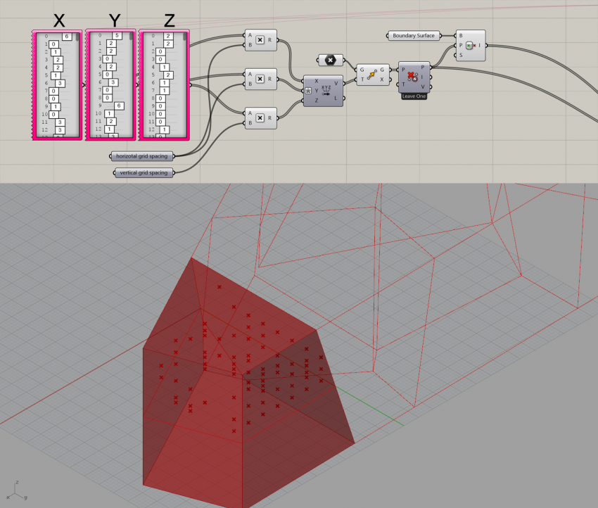
The voxelization has been accomplished in Grasshopper. The algorithm was fed by a list of generic three dimensional vectors (representing the generic points of a rectangular grid), a spatial domain (representing our voronoi cell) and the dimensions of the single voxel. The result was a transformed list of the input vectors obtained by deforming it and culling all duplicate vectors or those that happened to be outside of the voronoi cell. By altering the components of the input list in a range of discrete, integer values, the algorithm is able to produce an unique set of voxels. Those voxels could be interpreted as one among all the possible distributions of mass inside the voronoi cell.
In order to optimize the performance of the analysis and the efficiency of the script, we decided to represent the cells as single voxels.
1.2 The analysis
The analysis of the set of voxels produced by the previous step has been the most challenging part of the task, both at the conceptual and computational level.
We had to come out with a series of quantitative values that could be used to score a particular configuration of voxels. At that stage we had identified four parameters that had to be kept in consideration during the analysis: the average solar irradiation of the surfaces, the distance between the single cells, the number of neighbouring cells that every cell had and the total population (amount) of cells.
1.2.1 The Solar analysis
In order to perform the solar analysis we "materialized" the voxels by assigning to every vector produced at the previous step a box that would roughly approximate each of our cells. At first we considered to use Autodesk Ecotect as the analysis engine, but we soon discovered that any implementation of it would have runned way to slow for our purposes, making it unfeasible to test a large enough variety of different configurations. This was partially due to the fact that every configuration had to be exported from grasshopper to the Ecotect software. We therefore looked for a custom integrated script that, while being less accurate, would have delivered a result in a fraction of the time required by Ecotect. Keeping in mind the peculiarities of the geometry to analyze, which substantially is a grid of identical boxes, we could apply some specific considerations.
An interesting insight came from the algorithms used in computer graphics for displaying lines: those are a family of highly optimized pieces of software that, given a canvas of pixels and the characteristics of a line to trace (like its starting point, direction and length) would determine how to display it on screen, i.e. which of the pixels would became black and which would remain white. In particular we studied the Xiaolin Wu's line algorithm, an efficient, thus simple algotithm broadly used to generate an antialiased line.
We had the idea that, If we were able to implement one of those algorithms for a 3d structure of voxels instead for a 2d array of pixels, we could trace from every cell of our given population a line parallel to the sunlight direction to analyze and assume it to be the "path" of shadow casted by that voxel. Since the line is generated by an anti-aliased line algorithm and has the same "thickness" of a voxel, we could interpret it's rendered form as the real shadow that affects all the voxels on its path: a voxel that happens to be completely black would indicate a cell completely in shadow; viceversa, a white voxel a cell unaffected by that shadow. Every value of gray in between would characterize a cell only partially shadowed (more or less according to the luminance of the voxel). By multiplying, voxel by voxel, all the values generated by all the rest of the voxels, we would obtain the total volumetric shadow map of the entire configuration. This map could be used to evaluate the solar performance of the given configuration, as, for example, by taking the mean value of this shadowing score for all the cells.
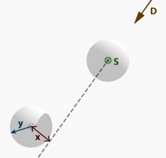
In practice, since an actual volumetric (over the classical 2d) implementation of the Xiaolin Wu's algorithms presented some difficulties we decide to trade off some of it's efficiency for the sake of code simplification. We have therefore proceeded implementing the same concept with a geometric approach achieved by minimizing the scripted parts while making a more extended use of standard grasshopper components.We proceed as follows: first, providing one or more significant solar directions as vectors, we generated form every center point of every voxel a line with that direction. We then calculated the distance of it from all the other center points. Those values were compared with a "radius" value that represented the radius of our cells cell. This means that if a given center point dists from the line previously calculated more than twice the radius, the voxel represented by that centerpoint would not receive any shadow from the voxel that casts the line, in the other case, it would appear shadowed in the proportion of it's distance compared to twice the radius. The image on the right shows a simplified model of this concept, where y represents the radius, x the distance between the center point and the line and D the solar direction. The relative amount of shadowing η that the cell A would receive from the cell B would be η=x/2y.
By superimposing all those scores calculated for every casted line on every voxel, we could obtain a map of the amount of shadow received by every cell. By this means we could assess the solar performance of a given cell configuration.
The first attempt of creating a component that could carry out an analysis in the fashion previously described is showed in the image above. The y parameter is the radius of the cell, S the centerpoint of the cell from which cast the shadow and D the considered direction of the sunlight as a vector. The VB.net component is a simple gate condition that outputs 1 if 2x>y, otherwhise it outputs 2x/y:
If 2x > y Then
     A = 1
   Else
     A = x / y
   End If
This is because, for the sake of this analysis, there is no difference if a given voxel is in not shadowed by a hair's breadth or by far. In this way, a voxel would get a score of 1 (that is fully lit) if the distance of its centerpoint form the axis of a given shadow is larger than the considered voxel radius, otherwise it gets, as score, the ratio between that distance and the radius. To make it clearer, a score of 0.5 indicates that the distance is the half of the radius, therefore the voxel is only lit by half.
Then, in order to sum the contribution of all the significant "shadow lines" on a given cell, we decide to consider, among all, only the two lines that were responsible of the highest shadowing score and adding their contribution taking into account their relative angle in relation to the cell; so, if the two lines affected the cell from the same side the contribution of the second over the first would be minimal (because the two shadows would mostly cover the same surface of the cell), in the other case their addition would be complete.
1.2.2 The distance score
In addition to the solar analysis we implemented a scoring system that forced the solution towards maximizing the average distance between the cells. This was dictated by the will of making the best use of all the volume available. This has been achieved by simply calculating all the distances between all the cells and obtaining the average of them.


